Neural Radiance Field!
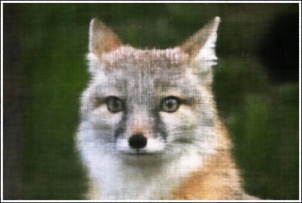
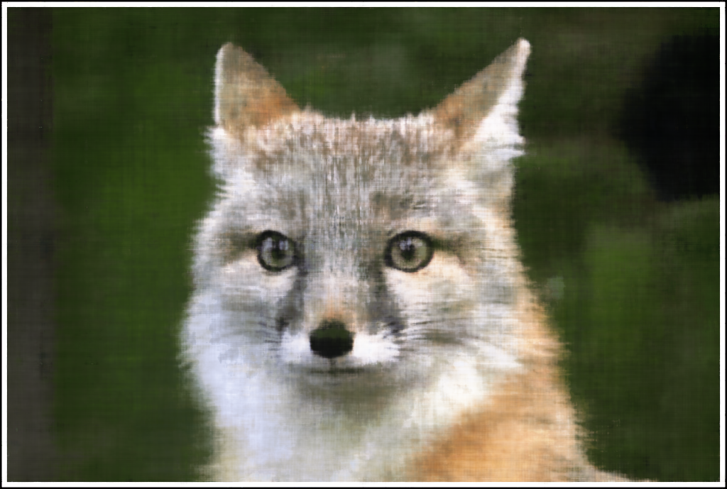
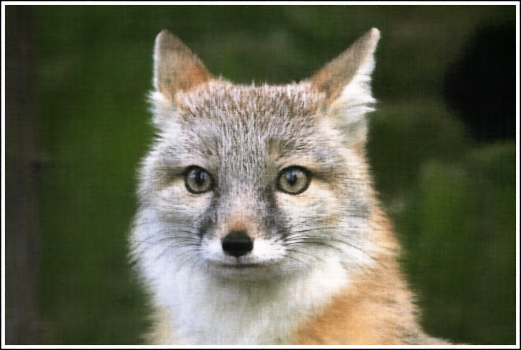
Part 1: Fit a Neural Field to a 2D Image
Network Architecture
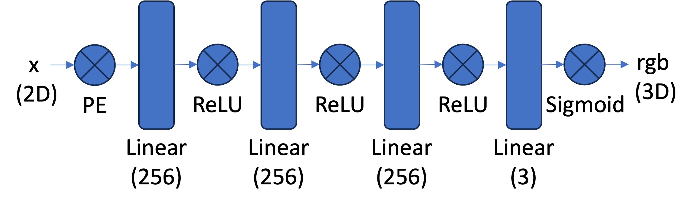
I created a multilayer perceptron (MLP) following the recommended
architecture. I used PyTorch and created an MLP with a custom
PositionalEncoding, linear layers interspersed with ReLU activations, and
a final sigmoid activation to ensure outputs are between 0 and 1.
The positional encoding is designed to expand the dimensionality of the
input, allowing the network to learn from different features at different
frequency levels. The following formula is used to calculate the
PositionalEncoding for both x and y coordinates.

Dataloader
I defined a training dataloader that randomly samples a batch_size of
N=10k coordinates and corresponding colors each time. I made sure to
normalize the coordinates and colors. To ensure that each batch is
different, I set the seed to the index of the batch before sampling.
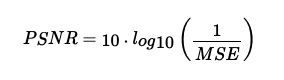
Training the MLP and Hyperparameter Tuning
I trained the MLP using MSE loss and Adam optimizer, running it for 3000
iterations. My hyperparameters included a max positional encoding
frequency of L = 10 and a channel size for the hidden layers of 256. For
hyperparameter tuning, I varied the number of hidden layers among 2, 3,
and 4, and I varied the learning rate among 0.1, 0.01, and 0.001. I used
the PSNR metric.
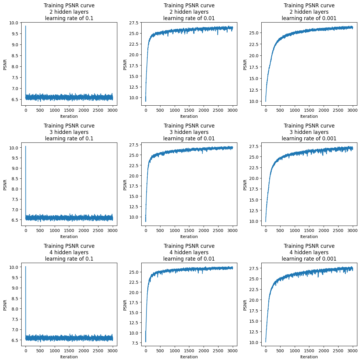
I plotted PSNR for both the fox and penguin over 3000 training iterations.
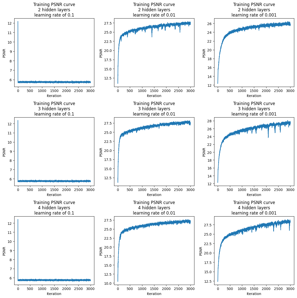
We can see that a learning rate of 0.1 performs abysmally, with a PSNR of
about 6 to 7. However, learning rates of 0.01 and 0.001 do well, reaching
PSNR of 25-28. The number of hidden layers does not have too much of an
influence. For the fox, here are the PSNR results:
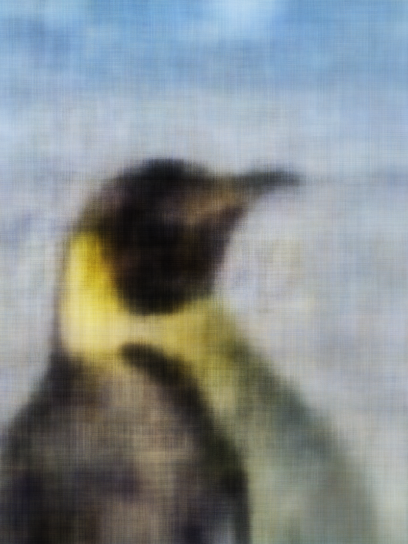
And for the penguin, here are the PSNR results:
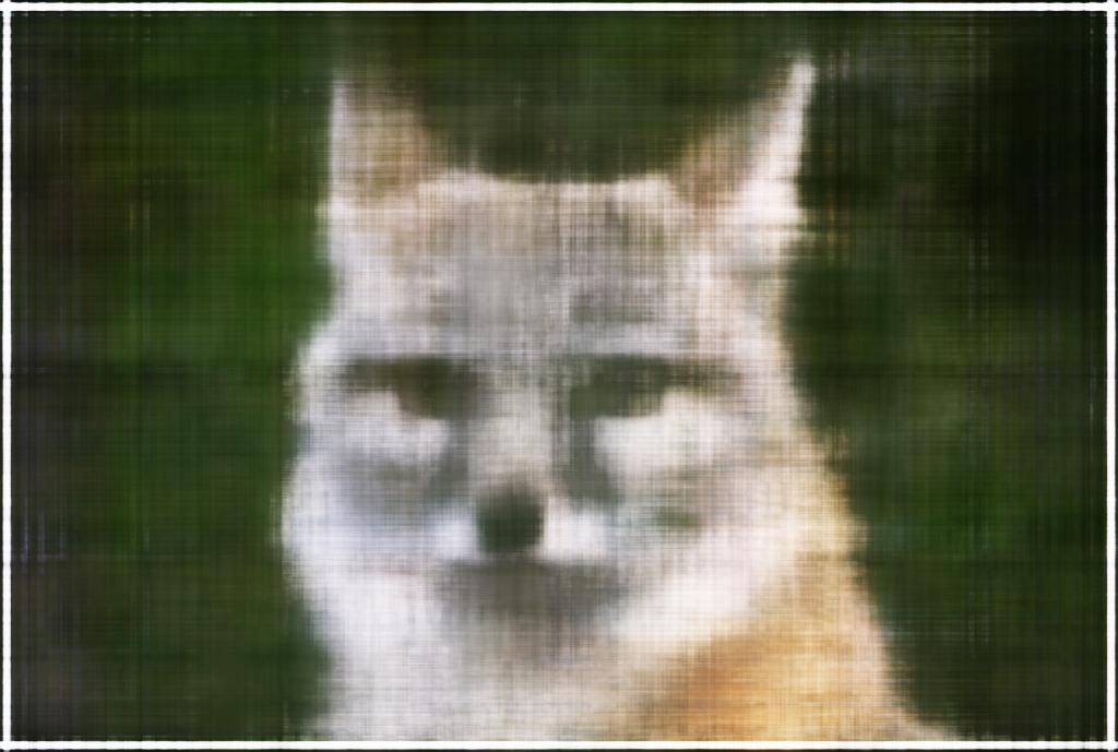
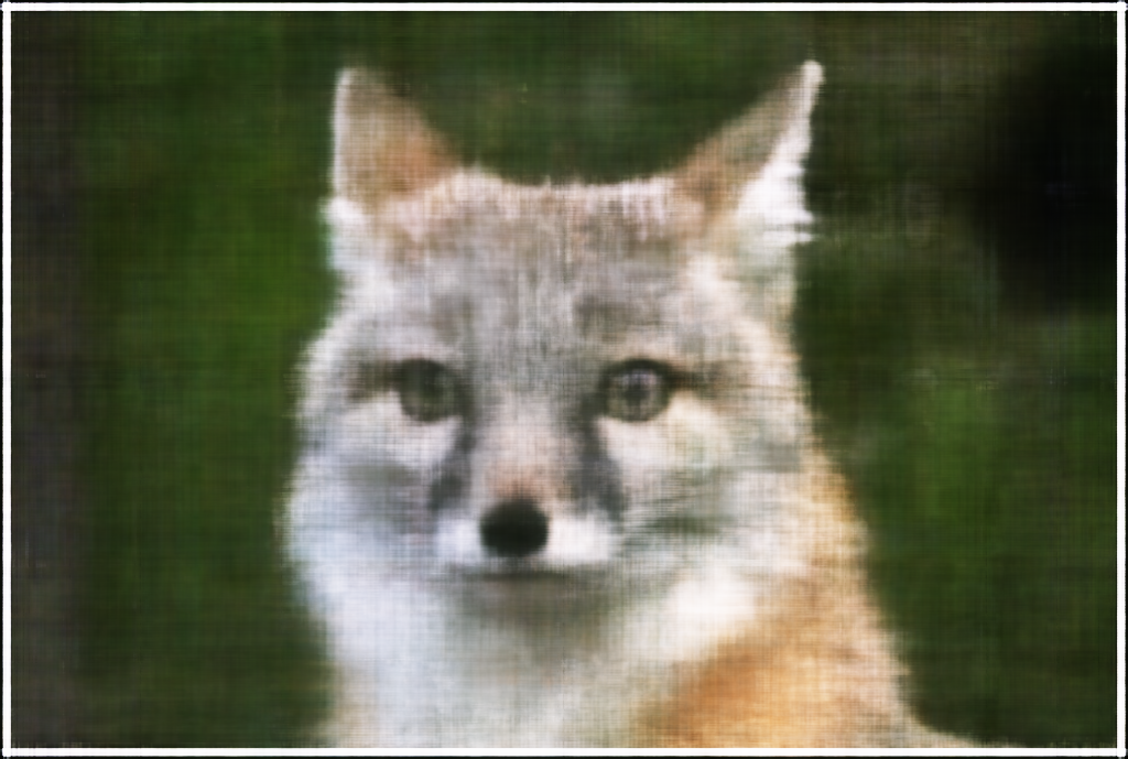
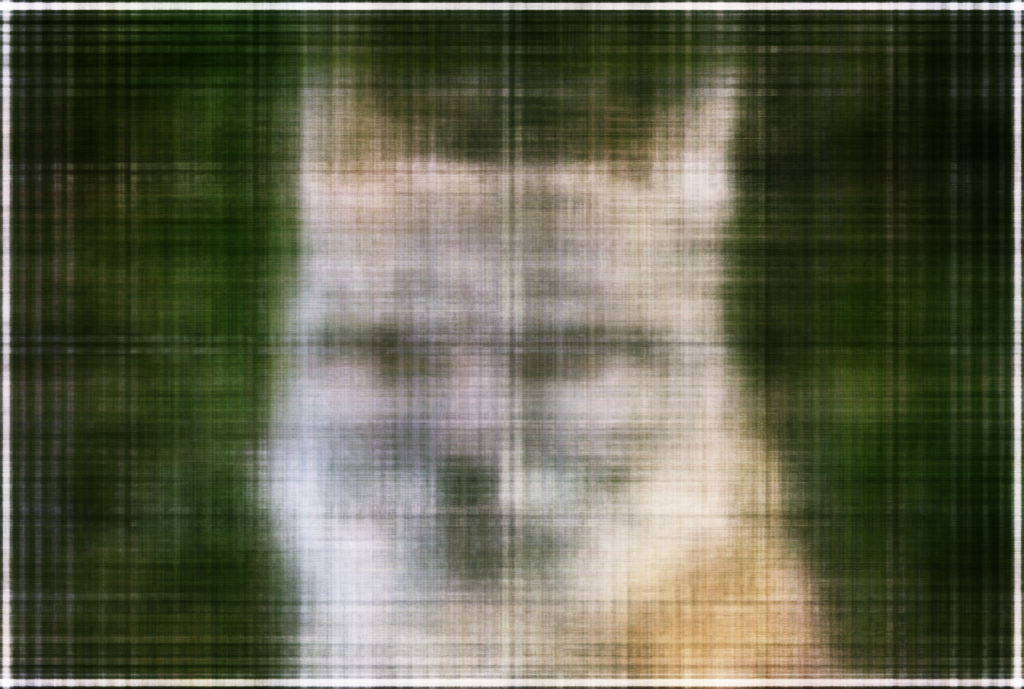
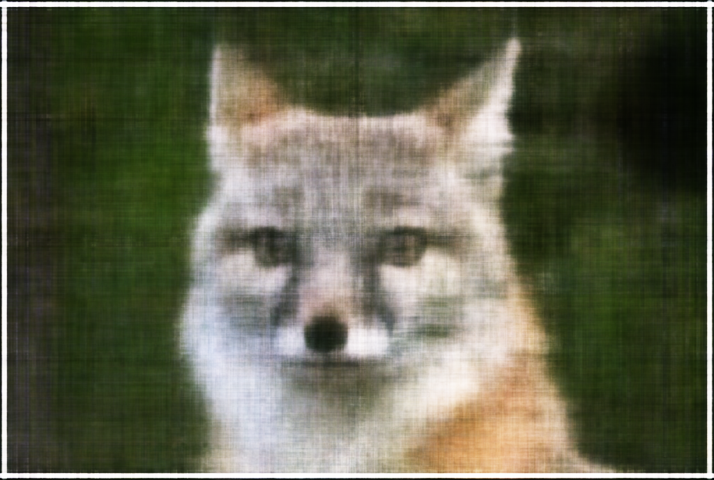
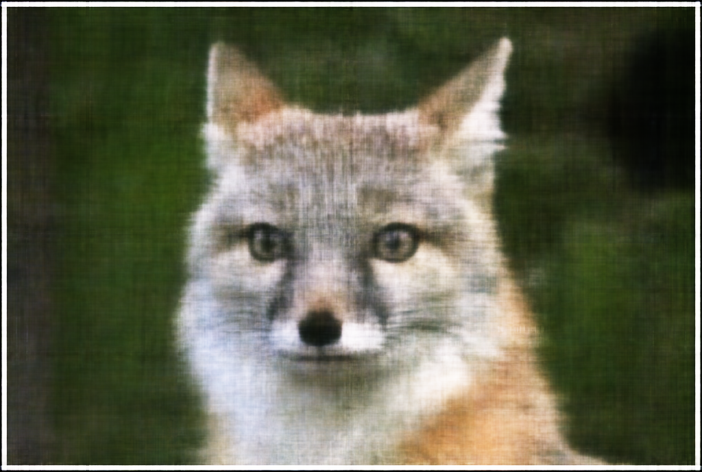
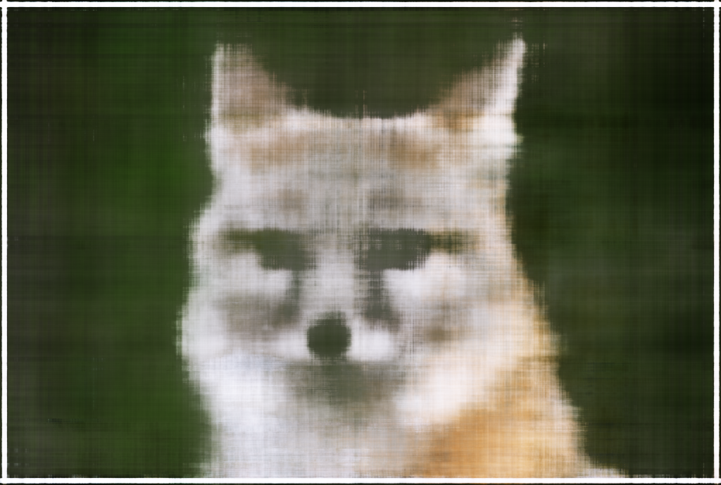
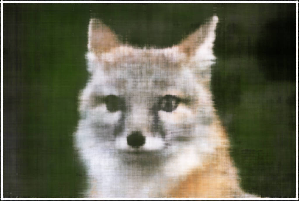
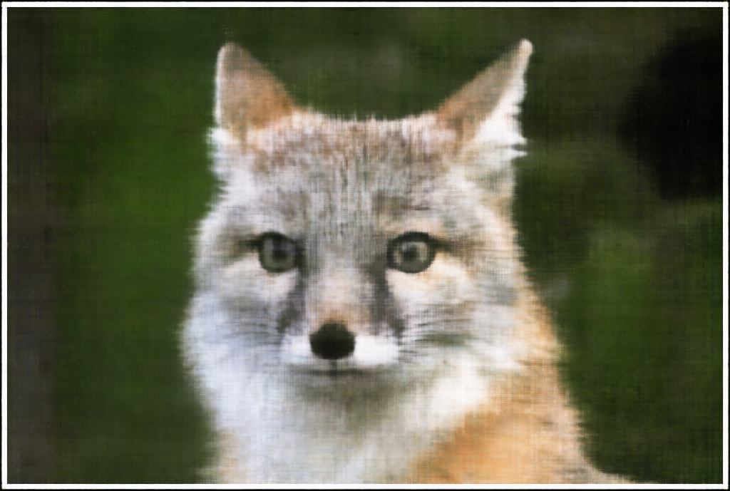
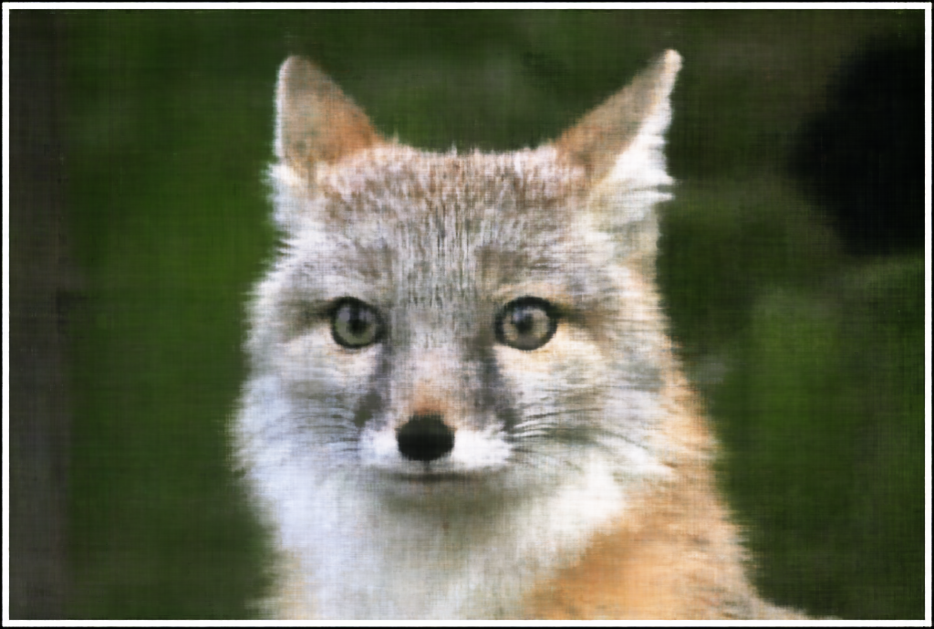
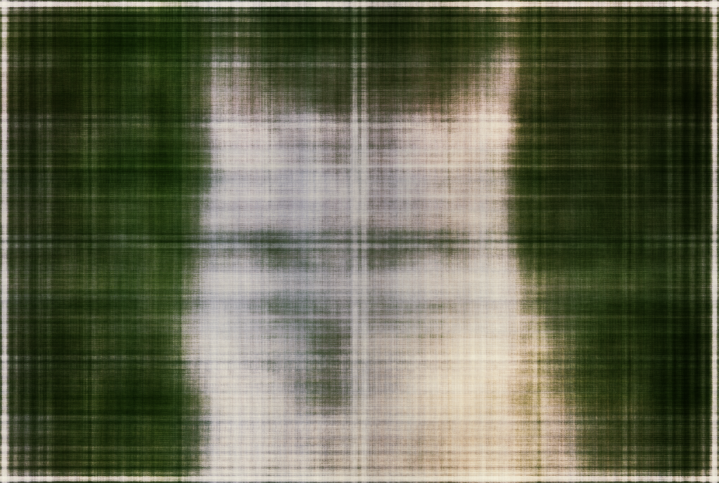
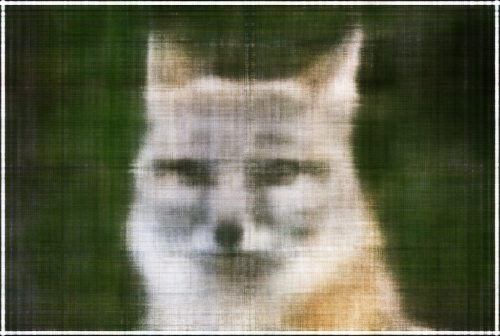
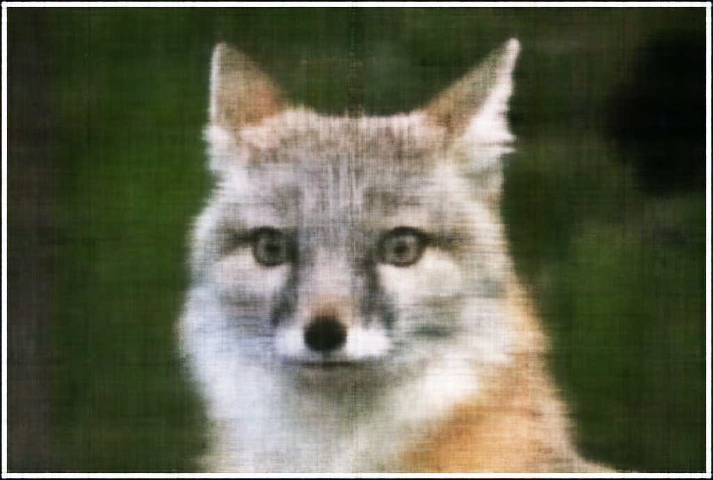
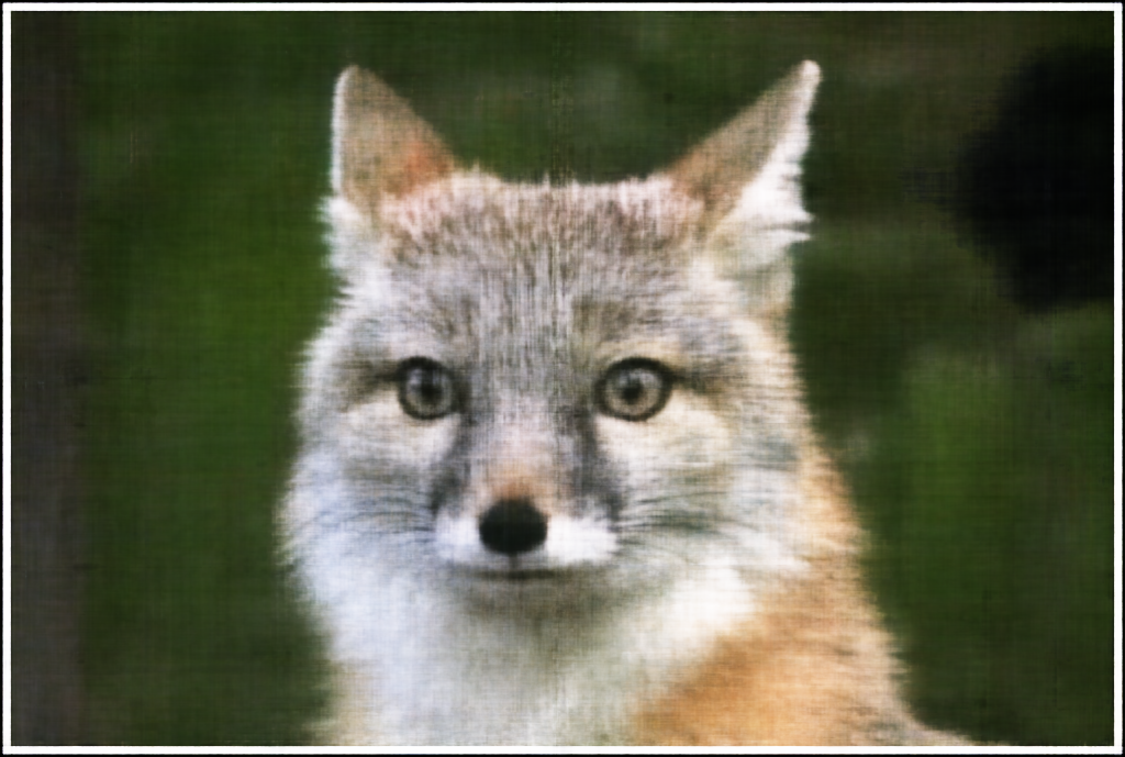
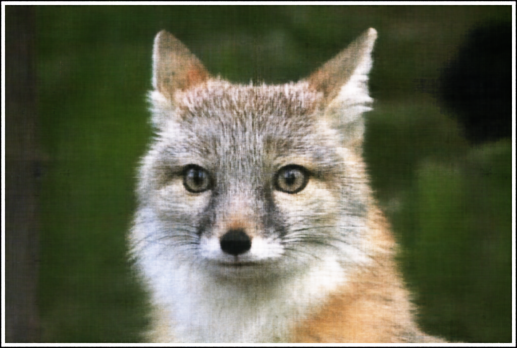
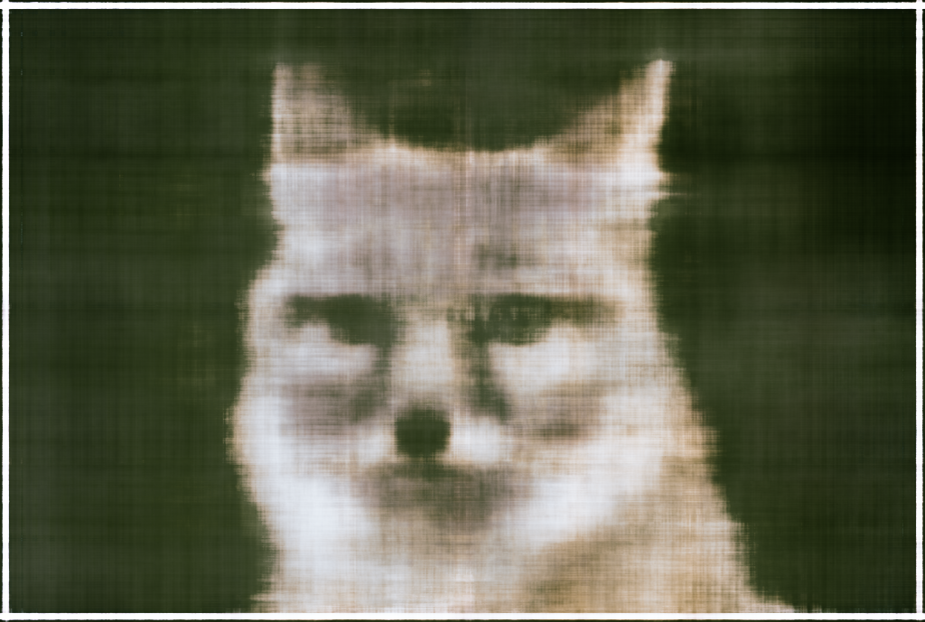
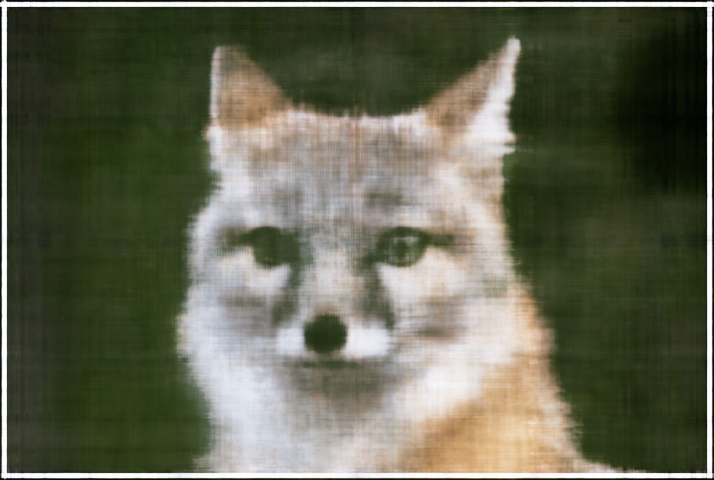
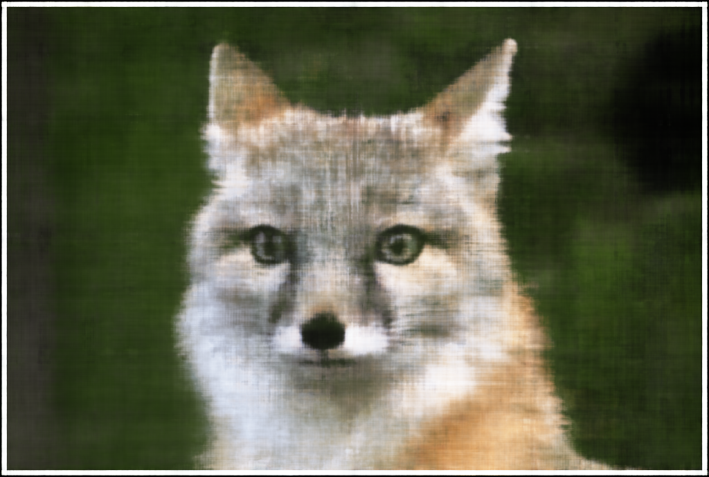
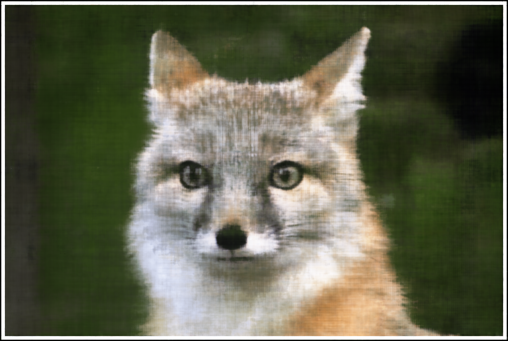
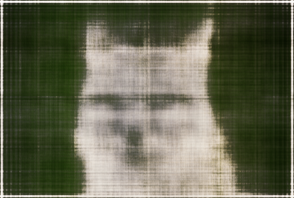
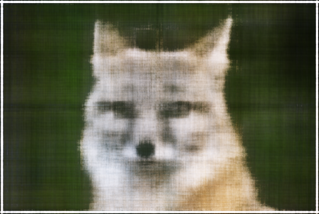
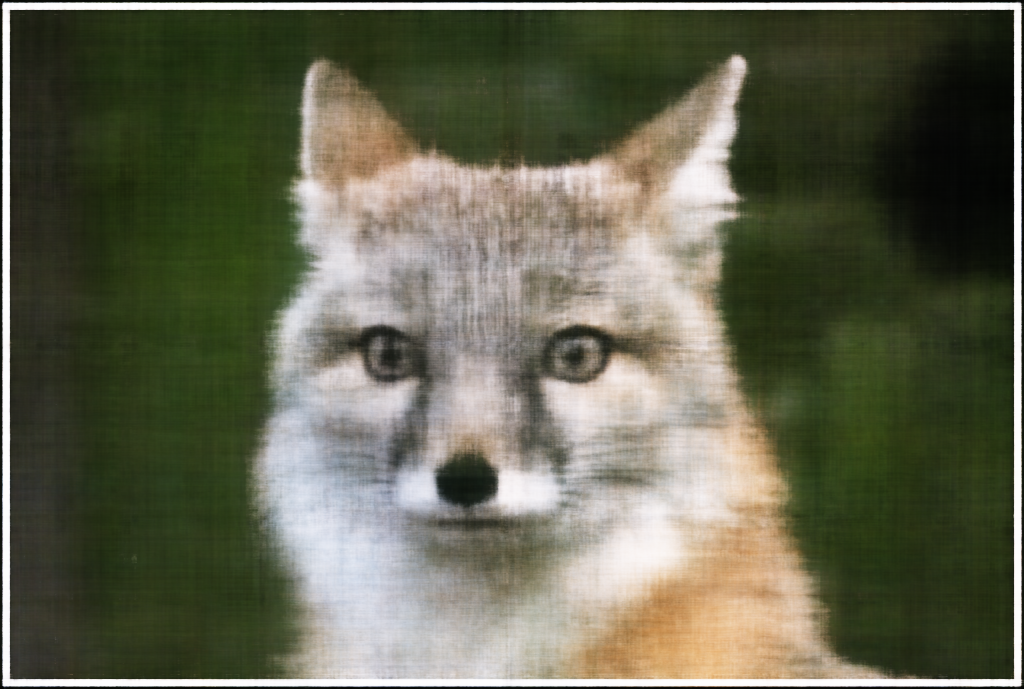
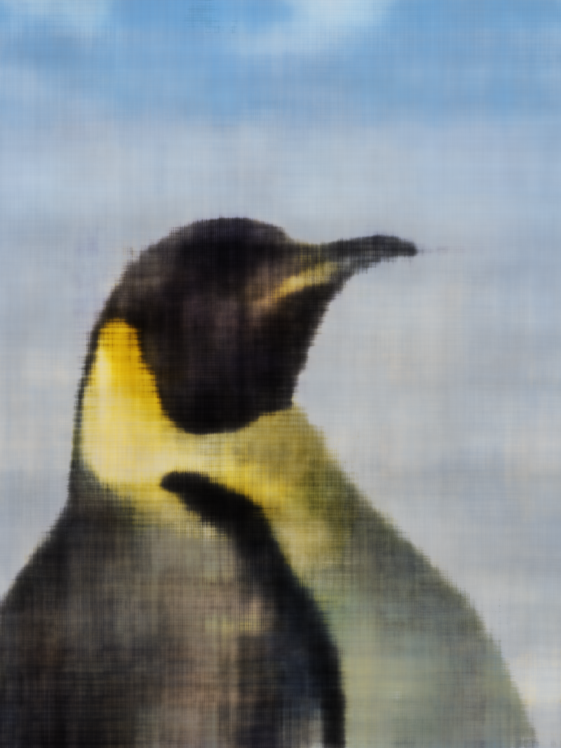
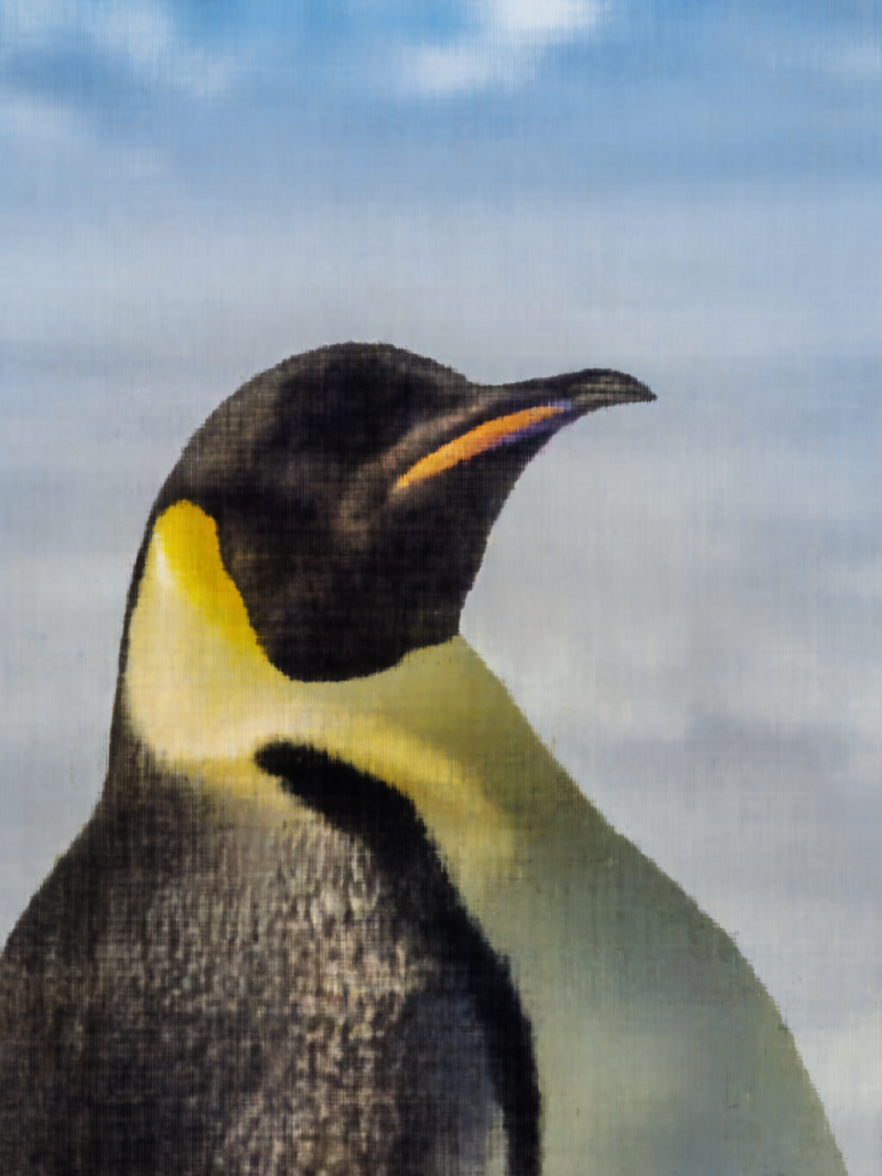
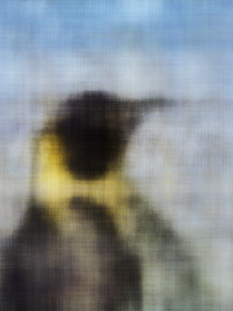
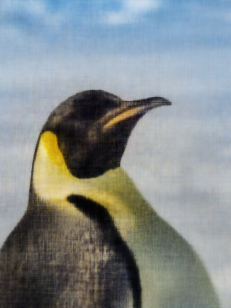
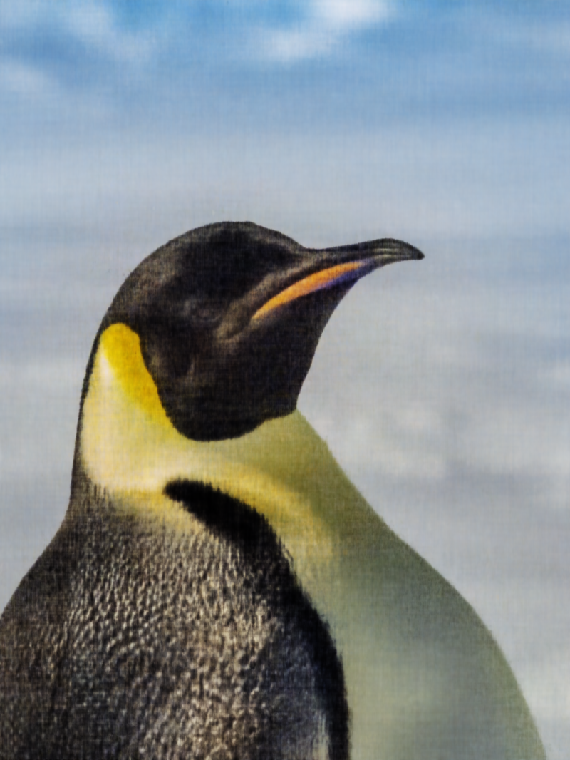
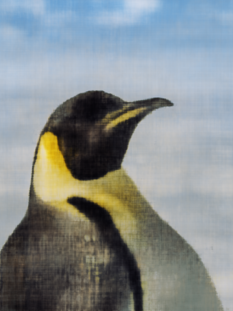
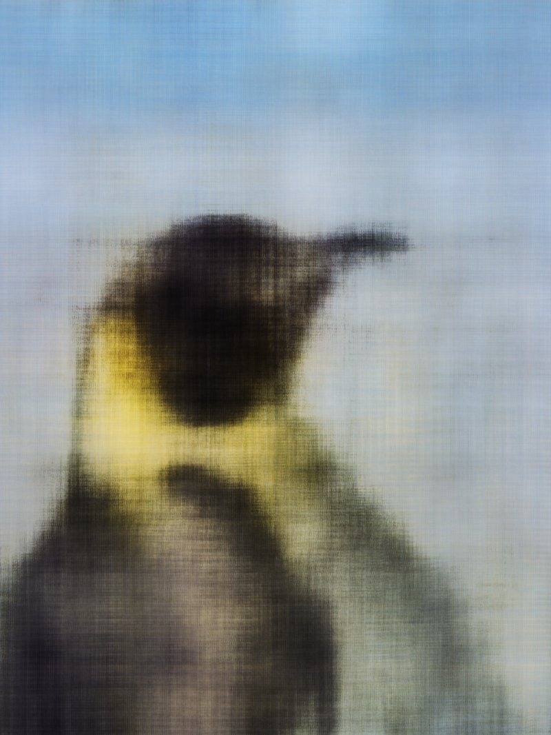
I visualized the training process over iterations 0, 100, 200, 600, 1500,
and the final 3000th iteration. I looked over 2, 3, and 4 hidden layers as
well as between 0.01 and 0.001 learning rates (0.1 did not seem to be a
good choice according to the PSNR curves). I can see that it appears that
lower learning rates do mean that the model takes longer to reach a clear
picture of the fox or penguin. In addition, increasing the number of
hidden layers seems to only slightly increase the detail and clarity of
the final iteration image, and may not be worth the increased overhead.
Part 2: Fit a Neural Radiance Field from Multi-view Images
Part 2.1: Create Rays from Cameras
Camera to World Coordinate Conversion
I defined a function called transform, which can take camera coordinates
and use a c2w transformation matrix to convert them to world coordinates.
I needed to make sure to convert the camera coordinates to 4D homogenous
coordinates first, and convert the world coordinates back to 3D Cartesian
coordinates.
Pixel to Camera Coordinate Conversion
I adapted the following formula:
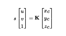
In order to calculate the camera coordinates, we can calculate s * K_inv *
uv. We again make sure to convert our uv 2D pixels into 3D homogenous
coordinates.
Pixel to Ray
We find the origin of the rays through the following formula:
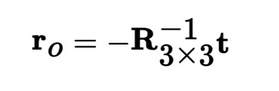
When finding R and t, we must extract these from the w2c matrix, which is
the inverse of the provided c2w matrices.
We then use the pixel to camera function as well as the camera to world
transform function in order to find the world coordinate (x_w)
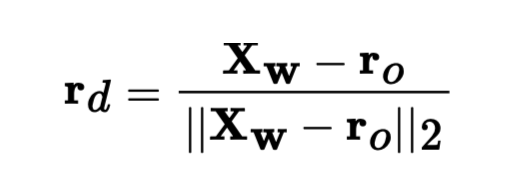
corresponding to the pixel at a depth of 1. Now that we have r_0 and x_w,
we can compute the normalized ray direction r_d, using the following
formula:
Part 2.2: Sampling
Sampling Rays from Images
We offset our coordinate grid by 0.5 to get the centers of the pixels. We
randomly sample batch_size pixels, and we use these pixels to get a ray
using our previous pixel to ray function. We go with the approach of
flattening all pixels and do a global sampling.
Sampling Points Along Rays
We sample points from the ray to discretize the continuous ray into 32
samples. We uniformly choose 32 different depths between near=2 and far=6,
and then we extract the points using the formula x = r_0 + r_d * t where t
are the uniformly chosen depths.
During training time, we also perturb the sampled points to reduce
overfitting. We do this by adding a small amount of random noise, so that
we no longer uniformly choose the depths of the sampled points. We use the
formula t += random noise * t_width, where t_width is set to 0.02.
Part 2.3: Putting the Dataloading All Together
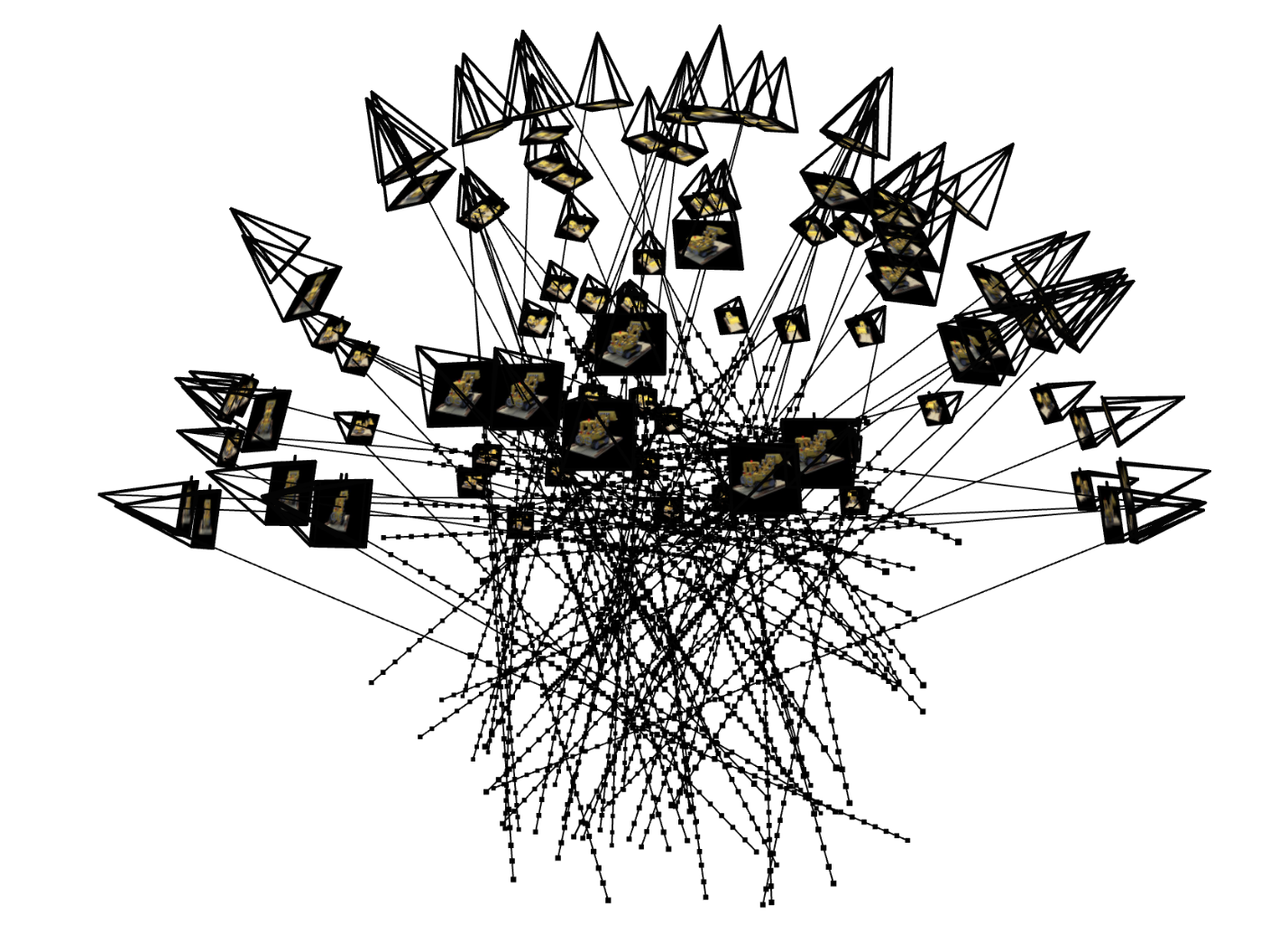
I used viser to visualize 100 rays, each with 32 points sampled. We can
see that each of the rays comes from a camera frustum (not all camera
frustums have rays coming out though), and the rays go towards the middle
which is likely the Lego set.
Part 2.4: Neural Radiance Field
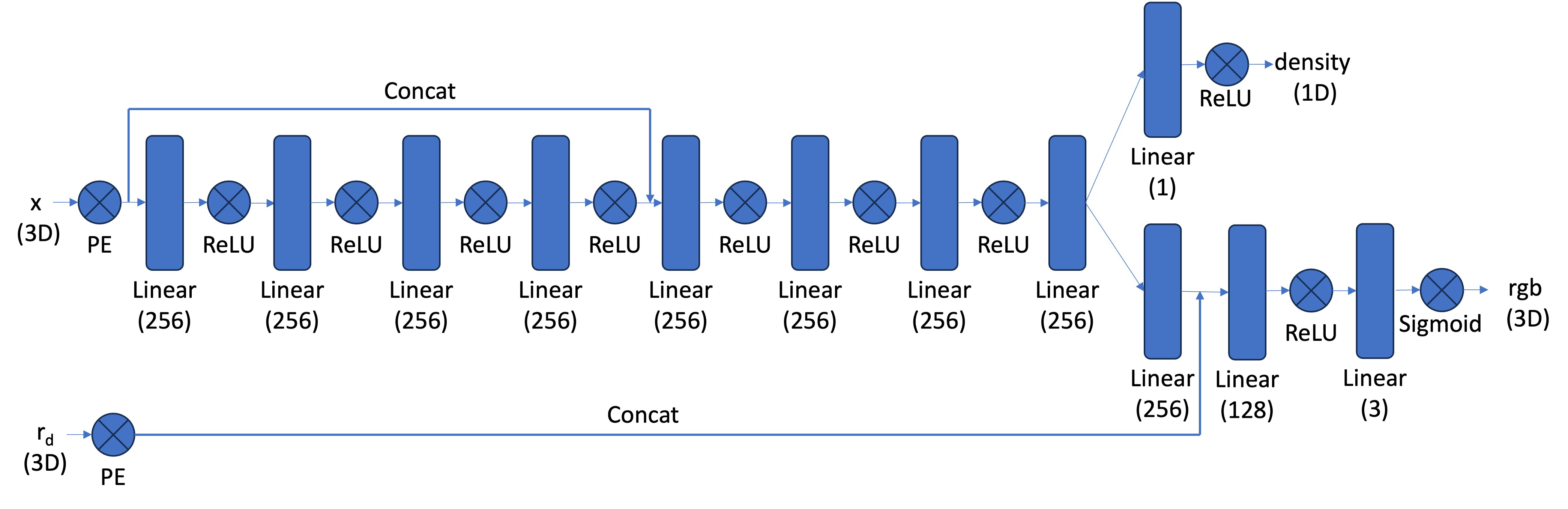
I used PyTorch to define an architecture. I followed the recommended
architecture. Smaller modules, like PositionalEncoding or a stack of
linear layers, definitely helped me to compose a complex architecture.
Part 2.5: Volume Rendering
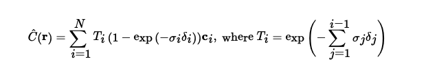
Our network outputs density and colors, and volume rendering helps us
determine the final color when the ray hits the image. At every step along
the ray (i.e., between different points sampled), we add the contribution
of that step to our color. Specifically, we use the following formula,
which takes into account the probability our ray terminates before or at
our sample location.
Training
We train using a batch size of 10k rays per gradient step as well as
n_samples=32 per ray. We also use an Adam optimizer with learning rate of
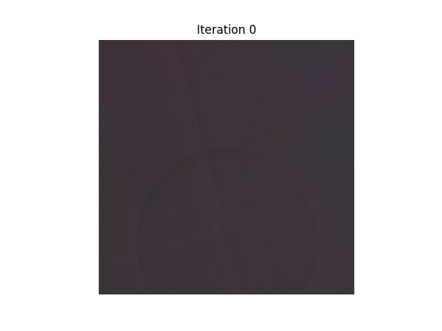
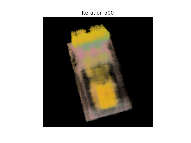
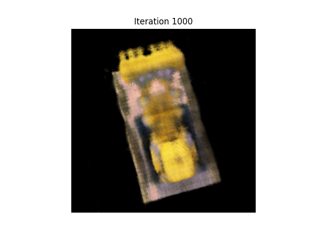
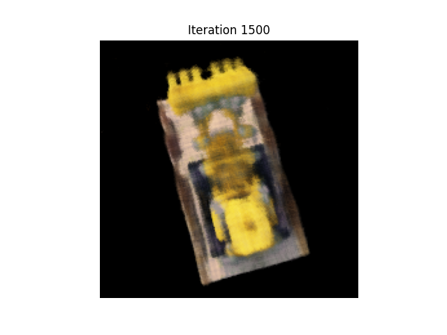
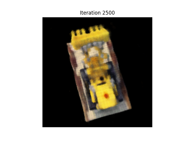
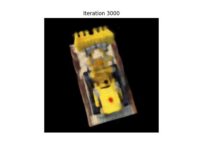
5e-4. We train for 3000 iterations. We can visualize the training process
across iterations, using the first camera extrinsics from the validation
dataset. Here, we see that the image gets clearer over time. We visualize
by using the validation camera extrinsics to get rays through each pixel
in our desired output image. We pass sampled points on this ray as well as
the ray direction into the NERF to get the output density and color, and
we use volume rendering to get our output image.
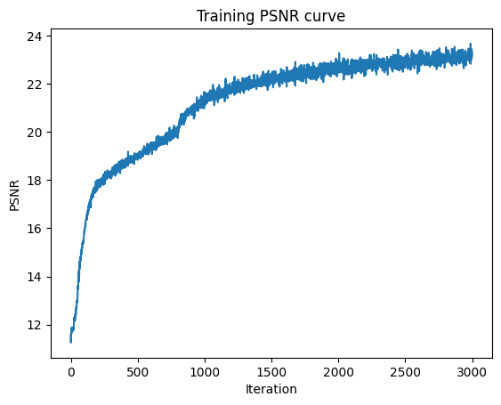
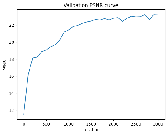
We can look at the PSNR over our training iterations, over both the
training batches and the validation dataset. We reach a PSNR of 23 after
3000 iterations.
When we use the provided test camera extrinsics, we can create a spherical
rendering of the lego video. We use the test camera extrinsics to get rays
through each pixel in our desired output image. We pass sampled points on
this ray as well as the ray direction into the NERF to get the output
density and color, and we use volume rendering to get our output image.
Bells and Whistles
Background color
We modify the volume rendering equation to add background color. Because
T_i is the probability of a ray not terminating before sample i, the
probability a ray does not terminate after all the samples (i.e., before
reaching the background) would be T_{n+1}. We can take T_{n+1} and
multiply by the injected background color (I chose red) and add that into
the pixel color. The idea is that the background color should show if
T_{n+1} is 1, which would be if the ray never passes through the Legos and
goes straight to the background.
Here is a GIF of the results.